A non-invasive method for concurrent detection of multiple early-stage cancers in women

Details of samples included in the study

The demographic and clinical information of samples included in the study are presented in Table 1 and Supplementary Table 1. The age distribution of these samples ranged from 20 to 90 years. Nearly 95% of the samples came from individuals between the ages of 30 to 80 years, and the remaining 5% was split between individuals from the age groups of 20—30 years and 81–90 years (Supplementary Fig. 1). The majority of samples (92%) were from Caucasian with only 8% of samples coming from non-White who were either Hispanic, Asian, or African American women. The total number of cancer samples was 1926, which included samples from women with either breast, endometrial, cervical, ovarian, lung, AML, thyroid, melanoma, colorectal, kidney, NHL, pancreatic, head & neck, gastric, liver and bile duct cancers. Additionally, we also included 300 samples from healthy volunteers as the normal control subset.

Pre-processing of data prior to AI workflow

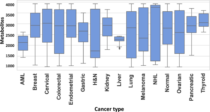
An untargeted metabolomics workflow involving positive ion mode ultra-pressure liquid chromatography coupled to mass spectrometry (UPLC-MS/MS) was employed for the individual serum samples described in Table-1. This resulted in > 20,000 spectral features (RT, m/z pairs), which was then further resolved into known metabolites by using the Human Metabolome Database (HMDB). The number of known metabolites obtained by this process for the individual groups of normal control, breast cancer, endometrial cancer, cervical cancer, ovarian cancer, lung cancer, AML, thyroid cancer, melanoma, colorectal cancer, kidney cancer, NHL, pancreatic cancer, head & neck cancer, gastric cancer and liver & bile duct cancer were 2821, 3119, 3209, 3237, 2638, 2238, 2215, 2344, 2622, 2117, 1935, 2033, 2202, 2160, 2116, and 2045, respectively. The cumulative list across all the groups was found to comprise of 8312 unique metabolites, which were then used for further analysis. The distribution of these unique metabolites across the individual sample groups is shown in Fig. 1. We next processed this data through our in-house pipeline that included normalization, gap filling, data transformation, followed by feature filtering and selection (Methods, Fig. 2) to generate a matrix consisting of 5104 features representing the 1926 cancer samples, as well as the 300 normal control samples.

Distribution of metabolites detected across the individual cancer groups. Figure provides a graphical distribution of the number of metabolites in the individual samples of each of the 15 cancer types included in the study. The cumulative number of named metabolites for all samples within a given cancer type is given in the text.

The data processing pipeline. The data processing approach used to develop the CDAI algorithm is illustrated here. Details are provided in the text.

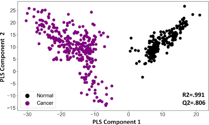
To determine whether the information contained in these features could distinguish between cancer samples and normal controls we first generated a PCA plot of cancer samples and normal controls with and without the QC samples. The initial plot was indicative for class separation (supplementary Fig. 2). Following this generated a PLSDA plot using the matrix. As shown in Fig. 3, the PLSDA plot could clearly differentiate cancer samples from normal control by segregating them into two distinct clusters (R2 = 0.991, Q2 = 0.806). To further develop this into a robust and sensitive method for cancer diagnosis, we resorted to AI analysis. The aim here was to more precisely capture variations in metabolite patterns that characterized the cancer samples on the one hand, and normal control samples on the other. In addition to cancer detection, we were also interested in developing an algorithm that enabled identification of the tissue of origin (TOO) in the case of cancer-positive samples. Accordingly then, we adopted a layered approach where we first focussed on accurately distinguishing cancer samples from the normal control, followed by the development of an algorithm for identifying the TOO of the cancer-positive samples.

PLSDA plot distinguishes cancer samples from normal controls. Results of a partial least squares-discriminant analysis (PLS-DA) is shown here as a plot of the matrix of samples and ion boxes versus metabolite intensity. The explained variation parameter R-squared parameter for cancer vs normal (R2 = 0.991). Q-squared value was evaluated using a separate test for the PLSDA fit which was equal to(Q2 = 0.8065).

Cancer detection artificial intelligence (CDAI) algorithm for distinguishing cancer samples from normal controls

The first step was to develop an algorithm for the differentiation of cancer samples from normal controls. We termed this as the Cancer Detection Artificial Intelligence (CDAI) model. For this, the matrix data was randomly divided into training and test sets in comparable proportion between the individual cancers and the normal controls in order to cumulatively distinguish all 15 cancers listed in Table 1 from normal controls. A total of 150 normal control samples and 966 cancer samples were used as the training set, while the test set was comprised of 150 normal controls and 960 cancer samples (Table 2). The accuracy, sensitivity, and specificity values for the CDAI model were obtained by applying it to the training set and evaluating it on the test set (Table 2 and Fig. 2). To distinguish between cancer samples and normal control, the logistic regression function was applied to the training data.

Here, × 0 is a constant number, I_i (1 ≤ i ≤ n) is the intensity of metabolite i present in the respective sample. The total number of metabolites is represented by the symbol n(n ∈ [1000, 5104]). Supplementary Fig. 3 gives the value of coefficient x_i(1 ≤ i ≤ n) for each metabolite.

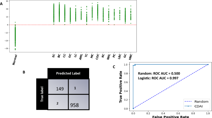
The model was cross validated across 1000 random train-test split which yielded an average sensitivity, specificity of 99.6 (99.5–99.8), 99.3 (98.9–99.5) at 95 CI respectively. The evaluation of the trained model as applied on a single test set for a single partition of data is shown in Fig. 4. The scatter plot in panel A shows the Model Score for normal controls and cancer cases. It is evident that these scores are clearly different between normal controls and the samples derived from all the different cancer types being tested (Fig. 4A). Application of a threshold of 0 to differentiate between cancer samples and normal controls resulted in the confusion matrix shown in Fig. 4B. From the results depicted in this matrix, the overall cancer detection sensitivity calculated was 99.7% whereas the specificity was 99.3%. The ROC-AUC curve obtained for the CDAI model results is also shown in Fig. 4C. The sensitivity of our CDAI algorithm for correctly identifying samples within each cancer type as cancer-positive is given in Table 3. It is evident from the results shown in this table that, barring one sample from the cervical cancer subset and another from the thyroid cancer subset, all other samples were correctly identified as cancer-positive. These results confirm that our pipeline of untargeted serum metabolomics coupled with data analysis using our CDAI algorithm provides for cancer detection with very high sensitivity and specificity. Importantly, given that the majority of samples across all 15 cancers were either from Stage-0 or Stage-I of the disease, the results in Table 3 also underscore the particular utility of our method for early-stage cancer detection.

The CDAI model accurately differentiates cancer samples from normal controls. (A) The results obtained with the trained CDAI model for cancer versus normal control samples in the test set. A scatter plot of the y-scores obtained for the individual samples within each of the cancer types is shown. The y-score of each of the 15 cancers are shown separately. The resulting confusion matrix obtained on applying a threshold of a y-score of 0 is shown in (B) wherein the high cancer detection accuracy—independent of the cancer type—is clearly evident. The precision of the CDAI algorithm was also confirmed by the ROC-AUC curve shown in Panel C, where the Area under ROC_AUC curve was 0.997. Individual cancer types are abbreviated in (A) as follows: BC breast cancer, EC endometrial cancer, CC cervical cancer, OC ovarian cancer, LC lung cancer, AML acute myeloid leukaemia, TC thyroid cancer, MC melanoma cancer, COC colorectal cancer, KC kidney cancer, NHL non-Hodgkin’s lymphoma, PC pancreatic cancer, HNC head and neck cancer, GC gastric cancer, LBC liver and bile duct cancer.

An artificial intelligence algorithm for determination of tissue of origin (TOOAI)

In the second step, our aim was to layer a multiclass AI model (tissue of origin, or, TOOAI model) on top of the CDAI model that would act on the cancer-positive samples from Table 3 to generate a multiclass score for each sample. That is, our aim was to score the relative probability with which the TOO of a given sample corresponded to each of the 15 cancer types that were being tested. Based on this grading then, it should be possible to identify the most likely TOO for that sample.

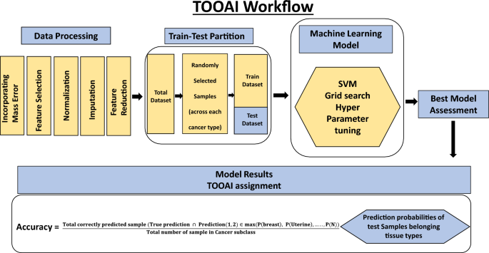
Our cumulative set of 1926 cancer samples included those from endometrial cancer (n = 304), breast cancer (n = 303), cervical cancer (n = 250), ovarian cancer (n = 262), lung cancer (n = 81), leukemia (n = 71), thyroid cancer (n = 70), melanoma (n = 86), colorectal cancer (n = 87), kidney cancer (n = 80), lymphoma (n = 50), pancreatic cancer (n = 75), liver & bile duct cancer (n = 34), gastric cancer (n = 85), head & neck cancer (n = 88). The matrix data generated for these samples was randomly partitioned into training and test datasets in equal proportion as shown in Fig. 5 and Table 4. Then, a SVM multiclass classification model was made using the training samples to generate the TOOAI algorithm. The TOOAI algorithm was applied on those samples identified as cancer-positive by the CDAI algorithm, which generated 15 scores for each sample. Here, for a given samples, each score defined the probability of that sample belonging to one of the fifteen classes, or cancer types.

The workflow employed for development of the TOOAI algorithm. The workflow for the multi cancer detection TOOAI platform involves three major compartments common to the layer model. These include model building, assessment of the models, and determination of double class prediction accuracy.

The multiclass classification TOOAI model was made using the training samples. The trained algorithm estimated tissue of origin probability of each of the sample, for each of the 15 cancer types, according to the formulae below:

Here, a₀, a₁, a₂,…., a_n are constant number, I_i (1 ≤ i ≤ 8312) is the Normalized intensity of metabolite i present in the respective sample. N is number of cancer type classes included in the training set.

The models were first assessed on the basis of their single class accuracy, wherein the first prediction (i.e. the highest probability score) was taken as the correct identification of the cancer TOO for a given sample. This analysis yielded an average accuracy across 15 cancers of 81% 95 CI (78.9–81.6) (results not shown). To further improve the accuracy, therefore, we considered a double-class prediction model in which the correct TOO likely occurred within the top two predictions from the model, calculated on the basis of the probability functions obtained as defined above. The double class prediction accuracies were evaluated for the test dataset and the confusion matrix for the final prediction is shown in Fig. 6. Double class prediction accuracy was obtained from the model by using the following formula:

Performance of the TOOAI model. The confusion matrix built for discriminating between the 15 cancers, on the basis of a double class TOO prediction accuracy, by the TOOAI model is shown here. Details of model development are provided in Methods while an interpretation of the results is discussed in the text. Individual cancer types are abbreviated as follows: BC breast cancer, EC endometrial cancer, CC cervical cancer, OC ovarian cancer, LC lung cancer, AML acute myeloid leukaemia, TC thyroid cancer, MC melanoma cancer, COC colorectal cancer, KC kidney cancer, NHL non-Hodgkin’s lymphoma, PC pancreatic cancer, HNC head and neck cancer, GC gastric cancer, LBC liver and bile duct cancer.

Table 5 gives the results obtained for the double class prediction analysis. The significant improvement in prediction accuracy is evident here, which ranged from a low of 82% for gastric cancer to as high as 100% for Non-Hodgkin’s lymphoma and pancreatic cancer. Of the total of 862 cancer samples that were tested, TOO of 795 were correctly predicted resulting in an average accuracy of 92.2% (Table 5).

Robustness of the CDAI

We also wanted to assess whether our method was subject to the vagaries of batch specific variability that is often seen in mass spectrometry data⁴⁶. For this, we performed an experiment using a sample set that comprised of a pre-defined number of samples from each of the 15 cancers and normal controls as shown in Table 6 and Supplementary Table 3. This sample set was subsequently analysed over multiple times at intervals of 4–6 weeks, spanning a total period of 18 months. Analysis involved a UPLC-MS/MS run for the individual samples, followed by determination of the cancer-positive versus cancer-negative status with the CDAI algorithm. A total of ten such test runs were performed and the results, in terms of the CDAI accuracy, are shown in Table 6 and illustrated in Supplementary Fig. 4. Importantly, the coefficient of variation for the net sensitivity for cancer detection obtained across these ten test runs was as low as 0.003 (Supplementary Fig. 4), confirming the robustness of our overall methodology. We believe that this is a significant finding from the standpoint of further development of our approach as a possible MCED test.

Identification of features critical for cancer detection

Our matrix features were able to recognize named metabolites in the HMDB database. This renders our model results more amenable towards gaining useful insights into the metabolic adaptations that seemingly correlate with cancer development. To facilitate such future analysis, we sought to short-list those metabolites that contributed significantly to the cancer-specific signatures detected by the CDAI algorithm. For this we employed feature ranking, wherein weights of the CDAI model’s individual features—or named metabolites—involved in distinguishing between cancer and normal control samples were first sorted. Subsequently, these features were ranked using the recursive feature elimination technique, which involved elimination of one feature at a time. The top ranking metabolites that resulted from this exercise are listed in Supplementary Table 2.